Chatbot Tutorial

Author: Matthew Inkawhich

In this tutorial, we explore a fun and interesting use-case of recurrent sequence-to-sequence models. We will train a simple chatbot using movie scripts from the Cornell Movie-Dialogs Corpus.

Conversational models are a hot topic in artificial intelligence research. Chatbots can be found in a variety of settings, including customer service applications and online helpdesks. These bots are often powered by retrieval-based models, which output predefined responses to questions of certain forms. In a highly restricted domain like a company’s IT helpdesk, these models may be sufficient, however, they are not robust enough for more general use-cases. Teaching a machine to carry out a meaningful conversation with a human in multiple domains is a research question that is far from solved. Recently, the deep learning boom has allowed for powerful generative models like Google’s Neural Conversational Model, which marks a large step towards multi-domain generative conversational models. In this tutorial, we will implement this kind of model in PyTorch.

> hello?
Bot: hello .
> where am I?
Bot: you re in a hospital .
> who are you?
Bot: i m a lawyer .
> how are you doing?
Bot: i m fine .
> are you my friend?
Bot: no .
> you're under arrest
Bot: i m trying to help you !
> i'm just kidding
Bot: i m sorry .
> where are you from?
Bot: san francisco .
> it's time for me to leave
Bot: i know .
> goodbye
Bot: goodbye .

Tutorial Highlights

• Handle loading and preprocessing of Cornell Movie-Dialogs Corpus dataset

• Implement a sequence-to-sequence model with Luong attention mechanism(s)

• Jointly train encoder and decoder models using mini-batches

• Implement greedy-search decoding module

• Interact with trained chatbot

Acknowledgements

This tutorial borrows code from the following sources:

1. Yuan-Kuei Wu’s pytorch-chatbot implementation: https://github.com/ywk991112/pytorch-chatbot

2. Sean Robertson’s practical-pytorch seq2seq-translation example: https://github.com/spro/practical-pytorch/tree/master/seq2seq-translation

3. FloydHub’s Cornell Movie Corpus preprocessing code: https://github.com/floydhub/textutil-preprocess-cornell-movie-corpus

Preparations

To start, Download the data ZIP file here and put in a data/ directory under the current directory.

After that, let’s import some necessities.

from __future__ import absolute_import
from __future__ import division
from __future__ import print_function
from __future__ import unicode_literals

import torch
from torch.jit import script, trace
import torch.nn as nn
from torch import optim
import torch.nn.functional as F
import csv
import random
import re
import os
import unicodedata
import codecs
from io import open
import itertools
import math


USE_CUDA = torch.cuda.is_available()
device = torch.device("cuda" if USE_CUDA else "cpu")

Load & Preprocess Data

The next step is to reformat our data file and load the data into structures that we can work with.

The Cornell Movie-Dialogs Corpus is a rich dataset of movie character dialog:

• 220,579 conversational exchanges between 10,292 pairs of movie characters

• 9,035 characters from 617 movies

• 304,713 total utterances

This dataset is large and diverse, and there is a great variation of language formality, time periods, sentiment, etc. Our hope is that this diversity makes our model robust to many forms of inputs and queries.

First, we’ll take a look at some lines of our datafile to see the original format.

corpus_name = "cornell movie-dialogs corpus"
corpus = os.path.join("data", corpus_name)

def printLines(file, n=10):
    with open(file, 'rb') as datafile:
        lines = datafile.readlines()
    for line in lines[:n]:
        print(line)

printLines(os.path.join(corpus, "movie_lines.txt"))

Create formatted data file

For convenience, we’ll create a nicely formatted data file in which each line contains a tab-separated query sentence and a response sentence pair.

The following functions facilitate the parsing of the raw movie_lines.txt data file.

• loadLines splits each line of the file into a dictionary of fields (lineID, characterID, movieID, character, text)

• loadConversations groups fields of lines from loadLines into conversations based on movie_conversations.txt

• extractSentencePairs extracts pairs of sentences from conversations

# Splits each line of the file into a dictionary of fields
def loadLines(fileName, fields):
    lines = {}
    with open(fileName, 'r', encoding='iso-8859-1') as f:
        for line in f:
            values = line.split(" +++$+++ ")
            # Extract fields
            lineObj = {}
            for i, field in enumerate(fields):
                lineObj[field] = values[i]
            lines[lineObj['lineID']] = lineObj
    return lines


# Groups fields of lines from `loadLines` into conversations based on *movie_conversations.txt*
def loadConversations(fileName, lines, fields):
    conversations = []
    with open(fileName, 'r', encoding='iso-8859-1') as f:
        for line in f:
            values = line.split(" +++$+++ ")
            # Extract fields
            convObj = {}
            for i, field in enumerate(fields):
                convObj[field] = values[i]
            # Convert string to list (convObj["utteranceIDs"] == "['L598485', 'L598486', ...]")
            utterance_id_pattern = re.compile('L[0-9]+')
            lineIds = utterance_id_pattern.findall(convObj["utteranceIDs"])
            # Reassemble lines
            convObj["lines"] = []
            for lineId in lineIds:
                convObj["lines"].append(lines[lineId])
            conversations.append(convObj)
    return conversations


# Extracts pairs of sentences from conversations
def extractSentencePairs(conversations):
    qa_pairs = []
    for conversation in conversations:
        # Iterate over all the lines of the conversation
        for i in range(len(conversation["lines"]) - 1):  # We ignore the last line (no answer for it)
            inputLine = conversation["lines"][i]["text"].strip()
            targetLine = conversation["lines"][i+1]["text"].strip()
            # Filter wrong samples (if one of the lists is empty)
            if inputLine and targetLine:
                qa_pairs.append([inputLine, targetLine])
    return qa_pairs

Now we’ll call these functions and create the file. We’ll call it formatted_movie_lines.txt.

# Define path to new file
datafile = os.path.join(corpus, "formatted_movie_lines.txt")

delimiter = '\t'
# Unescape the delimiter
delimiter = str(codecs.decode(delimiter, "unicode_escape"))

# Initialize lines dict, conversations list, and field ids
lines = {}
conversations = []
MOVIE_LINES_FIELDS = ["lineID", "characterID", "movieID", "character", "text"]
MOVIE_CONVERSATIONS_FIELDS = ["character1ID", "character2ID", "movieID", "utteranceIDs"]

# Load lines and process conversations
print("\nProcessing corpus...")
lines = loadLines(os.path.join(corpus, "movie_lines.txt"), MOVIE_LINES_FIELDS)
print("\nLoading conversations...")
conversations = loadConversations(os.path.join(corpus, "movie_conversations.txt"),
                                  lines, MOVIE_CONVERSATIONS_FIELDS)

# Write new csv file
print("\nWriting newly formatted file...")
with open(datafile, 'w', encoding='utf-8') as outputfile:
    writer = csv.writer(outputfile, delimiter=delimiter, lineterminator='\n')
    for pair in extractSentencePairs(conversations):
        writer.writerow(pair)

# Print a sample of lines
print("\nSample lines from file:")
printLines(datafile)

Load and trim data

Our next order of business is to create a vocabulary and load query/response sentence pairs into memory.

Note that we are dealing with sequences of words, which do not have an implicit mapping to a discrete numerical space. Thus, we must create one by mapping each unique word that we encounter in our dataset to an index value.

For this we define a Voc class, which keeps a mapping from words to indexes, a reverse mapping of indexes to words, a count of each word and a total word count. The class provides methods for adding a word to the vocabulary (addWord), adding all words in a sentence (addSentence) and trimming infrequently seen words (trim). More on trimming later.

# Default word tokens
PAD_token = 0  # Used for padding short sentences
SOS_token = 1  # Start-of-sentence token
EOS_token = 2  # End-of-sentence token

class Voc:
    def __init__(self, name):
        self.name = name
        self.trimmed = False
        self.word2index = {}
        self.word2count = {}
        self.index2word = {PAD_token: "PAD", SOS_token: "SOS", EOS_token: "EOS"}
        self.num_words = 3  # Count SOS, EOS, PAD

    def addSentence(self, sentence):
        for word in sentence.split(' '):
            self.addWord(word)

    def addWord(self, word):
        if word not in self.word2index:
            self.word2index[word] = self.num_words
            self.word2count[word] = 1
            self.index2word[self.num_words] = word
            self.num_words += 1
        else:
            self.word2count[word] += 1

    # Remove words below a certain count threshold
    def trim(self, min_count):
        if self.trimmed:
            return
        self.trimmed = True

        keep_words = []

        for k, v in self.word2count.items():
            if v >= min_count:
                keep_words.append(k)

        print('keep_words {} / {} = {:.4f}'.format(
            len(keep_words), len(self.word2index), len(keep_words) / len(self.word2index)
        ))

        # Reinitialize dictionaries
        self.word2index = {}
        self.word2count = {}
        self.index2word = {PAD_token: "PAD", SOS_token: "SOS", EOS_token: "EOS"}
        self.num_words = 3 # Count default tokens

        for word in keep_words:
            self.addWord(word)

Now we can assemble our vocabulary and query/response sentence pairs. Before we are ready to use this data, we must perform some preprocessing.

First, we must convert the Unicode strings to ASCII using unicodeToAscii. Next, we should convert all letters to lowercase and trim all non-letter characters except for basic punctuation (normalizeString). Finally, to aid in training convergence, we will filter out sentences with length greater than the MAX_LENGTH threshold (filterPairs).

MAX_LENGTH = 10  # Maximum sentence length to consider

# Turn a Unicode string to plain ASCII, thanks to
# https://stackoverflow.com/a/518232/2809427
def unicodeToAscii(s):
    return ''.join(
        c for c in unicodedata.normalize('NFD', s)
        if unicodedata.category(c) != 'Mn'
    )

# Lowercase, trim, and remove non-letter characters
def normalizeString(s):
    s = unicodeToAscii(s.lower().strip())
    s = re.sub(r"([.!?])", r" \1", s)
    s = re.sub(r"[^a-zA-Z.!?]+", r" ", s)
    s = re.sub(r"\s+", r" ", s).strip()
    return s

# Read query/response pairs and return a voc object
def readVocs(datafile, corpus_name):
    print("Reading lines...")
    # Read the file and split into lines
    lines = open(datafile, encoding='utf-8').\
        read().strip().split('\n')
    # Split every line into pairs and normalize
    pairs = [[normalizeString(s) for s in l.split('\t')] for l in lines]
    voc = Voc(corpus_name)
    return voc, pairs

# Returns True iff both sentences in a pair 'p' are under the MAX_LENGTH threshold
def filterPair(p):
    # Input sequences need to preserve the last word for EOS token
    return len(p[0].split(' ')) < MAX_LENGTH and len(p[1].split(' ')) < MAX_LENGTH

# Filter pairs using filterPair condition
def filterPairs(pairs):
    return [pair for pair in pairs if filterPair(pair)]

# Using the functions defined above, return a populated voc object and pairs list
def loadPrepareData(corpus, corpus_name, datafile, save_dir):
    print("Start preparing training data ...")
    voc, pairs = readVocs(datafile, corpus_name)
    print("Read {!s} sentence pairs".format(len(pairs)))
    pairs = filterPairs(pairs)
    print("Trimmed to {!s} sentence pairs".format(len(pairs)))
    print("Counting words...")
    for pair in pairs:
        voc.addSentence(pair[0])
        voc.addSentence(pair[1])
    print("Counted words:", voc.num_words)
    return voc, pairs


# Load/Assemble voc and pairs
save_dir = os.path.join("data", "save")
voc, pairs = loadPrepareData(corpus, corpus_name, datafile, save_dir)
# Print some pairs to validate
print("\npairs:")
for pair in pairs[:10]:
    print(pair)

Another tactic that is beneficial to achieving faster convergence during training is trimming rarely used words out of our vocabulary. Decreasing the feature space will also soften the difficulty of the function that the model must learn to approximate. We will do this as a two-step process:

1. Trim words used under MIN_COUNT threshold using the voc.trim function.

2. Filter out pairs with trimmed words.

MIN_COUNT = 3    # Minimum word count threshold for trimming

def trimRareWords(voc, pairs, MIN_COUNT):
    # Trim words used under the MIN_COUNT from the voc
    voc.trim(MIN_COUNT)
    # Filter out pairs with trimmed words
    keep_pairs = []
    for pair in pairs:
        input_sentence = pair[0]
        output_sentence = pair[1]
        keep_input = True
        keep_output = True
        # Check input sentence
        for word in input_sentence.split(' '):
            if word not in voc.word2index:
                keep_input = False
                break
        # Check output sentence
        for word in output_sentence.split(' '):
            if word not in voc.word2index:
                keep_output = False
                break

        # Only keep pairs that do not contain trimmed word(s) in their input or output sentence
        if keep_input and keep_output:
            keep_pairs.append(pair)

    print("Trimmed from {} pairs to {}, {:.4f} of total".format(len(pairs), len(keep_pairs), len(keep_pairs) / len(pairs)))
    return keep_pairs


# Trim voc and pairs
pairs = trimRareWords(voc, pairs, MIN_COUNT)

Prepare Data for Models

Although we have put a great deal of effort into preparing and massaging our data into a nice vocabulary object and list of sentence pairs, our models will ultimately expect numerical torch tensors as inputs. One way to prepare the processed data for the models can be found in the seq2seq translation tutorial. In that tutorial, we use a batch size of 1, meaning that all we have to do is convert the words in our sentence pairs to their corresponding indexes from the vocabulary and feed this to the models.

However, if you’re interested in speeding up training and/or would like to leverage GPU parallelization capabilities, you will need to train with mini-batches.

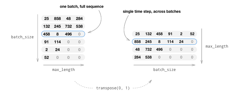
Using mini-batches also means that we must be mindful of the variation of sentence length in our batches. To accomodate sentences of different sizes in the same batch, we will make our batched input tensor of shape (max_length, batch_size), where sentences shorter than the max_length are zero padded after an EOS_token.

If we simply convert our English sentences to tensors by converting words to their indexes(indexesFromSentence) and zero-pad, our tensor would have shape (batch_size, max_length) and indexing the first dimension would return a full sequence across all time-steps. However, we need to be able to index our batch along time, and across all sequences in the batch. Therefore, we transpose our input batch shape to (max_length, batch_size), so that indexing across the first dimension returns a time step across all sentences in the batch. We handle this transpose implicitly in the zeroPadding function.

The inputVar function handles the process of converting sentences to tensor, ultimately creating a correctly shaped zero-padded tensor. It also returns a tensor of lengths for each of the sequences in the batch which will be passed to our decoder later.

The outputVar function performs a similar function to inputVar, but instead of returning a lengths tensor, it returns a binary mask tensor and a maximum target sentence length. The binary mask tensor has the same shape as the output target tensor, but every element that is a PAD_token is 0 and all others are 1.

batch2TrainData simply takes a bunch of pairs and returns the input and target tensors using the aforementioned functions.

def indexesFromSentence(voc, sentence):
    return [voc.word2index[word] for word in sentence.split(' ')] + [EOS_token]


def zeroPadding(l, fillvalue=PAD_token):
    return list(itertools.zip_longest(*l, fillvalue=fillvalue))

def binaryMatrix(l, value=PAD_token):
    m = []
    for i, seq in enumerate(l):
        m.append([])
        for token in seq:
            if token == PAD_token:
                m[i].append(0)
            else:
                m[i].append(1)
    return m

# Returns padded input sequence tensor and lengths
def inputVar(l, voc):
    indexes_batch = [indexesFromSentence(voc, sentence) for sentence in l]
    lengths = torch.tensor([len(indexes) for indexes in indexes_batch])
    padList = zeroPadding(indexes_batch)
    padVar = torch.LongTensor(padList)
    return padVar, lengths

# Returns padded target sequence tensor, padding mask, and max target length
def outputVar(l, voc):
    indexes_batch = [indexesFromSentence(voc, sentence) for sentence in l]
    max_target_len = max([len(indexes) for indexes in indexes_batch])
    padList = zeroPadding(indexes_batch)
    mask = binaryMatrix(padList)
    mask = torch.ByteTensor(mask)
    padVar = torch.LongTensor(padList)
    return padVar, mask, max_target_len

# Returns all items for a given batch of pairs
def batch2TrainData(voc, pair_batch):
    pair_batch.sort(key=lambda x: len(x[0].split(" ")), reverse=True)
    input_batch, output_batch = [], []
    for pair in pair_batch:
        input_batch.append(pair[0])
        output_batch.append(pair[1])
    inp, lengths = inputVar(input_batch, voc)
    output, mask, max_target_len = outputVar(output_batch, voc)
    return inp, lengths, output, mask, max_target_len


# Example for validation
small_batch_size = 5
batches = batch2TrainData(voc, [random.choice(pairs) for _ in range(small_batch_size)])
input_variable, lengths, target_variable, mask, max_target_len = batches

print("input_variable:", input_variable)
print("lengths:", lengths)
print("target_variable:", target_variable)
print("mask:", mask)
print("max_target_len:", max_target_len)

Define Models

Seq2Seq Model

The brains of our chatbot is a sequence-to-sequence (seq2seq) model. The goal of a seq2seq model is to take a variable-length sequence as an input, and return a variable-length sequence as an output using a fixed-sized model.

Sutskever et al. discovered that by using two separate recurrent neural nets together, we can accomplish this task. One RNN acts as an encoder, which encodes a variable length input sequence to a fixed-length context vector. In theory, this context vector (the final hidden layer of the RNN) will contain semantic information about the query sentence that is input to the bot. The second RNN is a decoder, which takes an input word and the context vector, and returns a guess for the next word in the sequence and a hidden state to use in the next iteration.

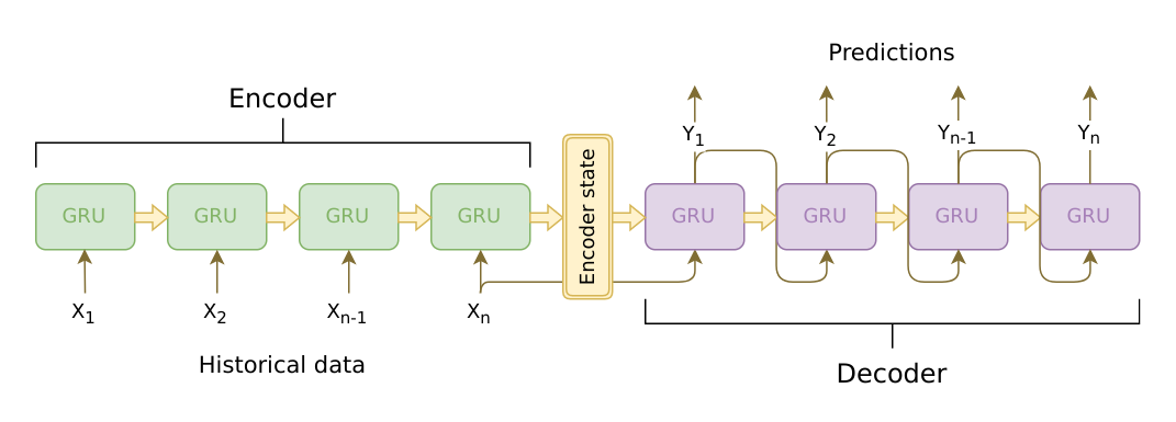
Image source: https://jeddy92.github.io/JEddy92.github.io/ts_seq2seq_intro/

Encoder

The encoder RNN iterates through the input sentence one token (e.g. word) at a time, at each time step outputting an “output” vector and a “hidden state” vector. The hidden state vector is then passed to the next time step, while the output vector is recorded. The encoder transforms the context it saw at each point in the sequence into a set of points in a high-dimensional space, which the decoder will use to generate a meaningful output for the given task.

At the heart of our encoder is a multi-layered Gated Recurrent Unit, invented by Cho et al. in 2014. We will use a bidirectional variant of the GRU, meaning that there are essentially two independent RNNs: one that is fed the input sequence in normal sequential order, and one that is fed the input sequence in reverse order. The outputs of each network are summed at each time step. Using a bidirectional GRU will give us the advantage of encoding both past and future context.

Bidirectional RNN:

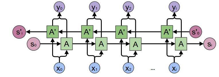
Image source: https://colah.github.io/posts/2015-09-NN-Types-FP/

Note that an embedding layer is used to encode our word indices in an arbitrarily sized feature space. For our models, this layer will map each word to a feature space of size hidden_size. When trained, these values should encode semantic similarity between similar meaning words.

Finally, if passing a padded batch of sequences to an RNN module, we must pack and unpack padding around the RNN pass using nn.utils.rnn.pack_padded_sequence and nn.utils.rnn.pad_packed_sequence respectively.

Computation Graph:

1. Convert word indexes to embeddings.

2. Pack padded batch of sequences for RNN module.

3. Forward pass through GRU.

4. Unpack padding.

5. Sum bidirectional GRU outputs.

6. Return output and final hidden state.

Inputs:

• input_seq: batch of input sentences; shape=(max_length, batch_size)

• input_lengths: list of sentence lengths corresponding to each sentence in the batch; shape=(batch_size)

• hidden: hidden state; shape=(n_layers x num_directions, batch_size, hidden_size)

Outputs:

• outputs: output features from the last hidden layer of the GRU (sum of bidirectional outputs); shape=(max_length, batch_size, hidden_size)

• hidden: updated hidden state from GRU; shape=(n_layers x num_directions, batch_size, hidden_size)

class EncoderRNN(nn.Module):
    def __init__(self, hidden_size, embedding, n_layers=1, dropout=0):
        super(EncoderRNN, self).__init__()
        self.n_layers = n_layers
        self.hidden_size = hidden_size
        self.embedding = embedding

        # Initialize GRU; the input_size and hidden_size params are both set to 'hidden_size'
        #   because our input size is a word embedding with number of features == hidden_size
        self.gru = nn.GRU(hidden_size, hidden_size, n_layers,
                          dropout=(0 if n_layers == 1 else dropout), bidirectional=True)

    def forward(self, input_seq, input_lengths, hidden=None):
        # Convert word indexes to embeddings
        embedded = self.embedding(input_seq)
        # Pack padded batch of sequences for RNN module
        packed = nn.utils.rnn.pack_padded_sequence(embedded, input_lengths)
        # Forward pass through GRU
        outputs, hidden = self.gru(packed, hidden)
        # Unpack padding
        outputs, _ = nn.utils.rnn.pad_packed_sequence(outputs)
        # Sum bidirectional GRU outputs
        outputs = outputs[:, :, :self.hidden_size] + outputs[:, : ,self.hidden_size:]
        # Return output and final hidden state
        return outputs, hidden

Decoder

The decoder RNN generates the response sentence in a token-by-token fashion. It uses the encoder’s context vectors, and internal hidden states to generate the next word in the sequence. It continues generating words until it outputs an EOS_token, representing the end of the sentence. A common problem with a vanilla seq2seq decoder is that if we rely soley on the context vector to encode the entire input sequence’s meaning, it is likely that we will have information loss. This is especially the case when dealing with long input sequences, greatly limiting the capability of our decoder.

To combat this, Bahdanau et al. created an “attention mechanism” that allows the decoder to pay attention to certain parts of the input sequence, rather than using the entire fixed context at every step.

At a high level, attention is calculated using the decoder’s current hidden state and the encoder’s outputs. The output attention weights have the same shape as the input sequence, allowing us to multiply them by the encoder outputs, giving us a weighted sum which indicates the parts of encoder output to pay attention to. Sean Robertson’s figure describes this very well:

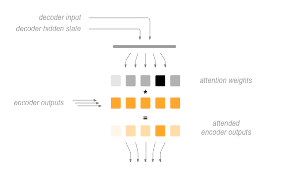
Luong et al. improved upon Bahdanau et al.’s groundwork by creating “Global attention”. The key difference is that with “Global attention”, we consider all of the encoder’s hidden states, as opposed to Bahdanau et al.’s “Local attention”, which only considers the encoder’s hidden state from the current time step. Another difference is that with “Global attention”, we calculate attention weights, or energies, using the hidden state of the decoder from the current time step only. Bahdanau et al.’s attention calculation requires knowledge of the decoder’s state from the previous time step. Also, Luong et al. provides various methods to calculate the attention energies between the encoder output and decoder output which are called “score functions”:

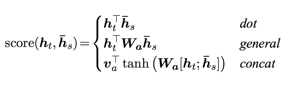
where \(h_t\) = current target decoder state and \(\bar{h}_s\) = all encoder states.

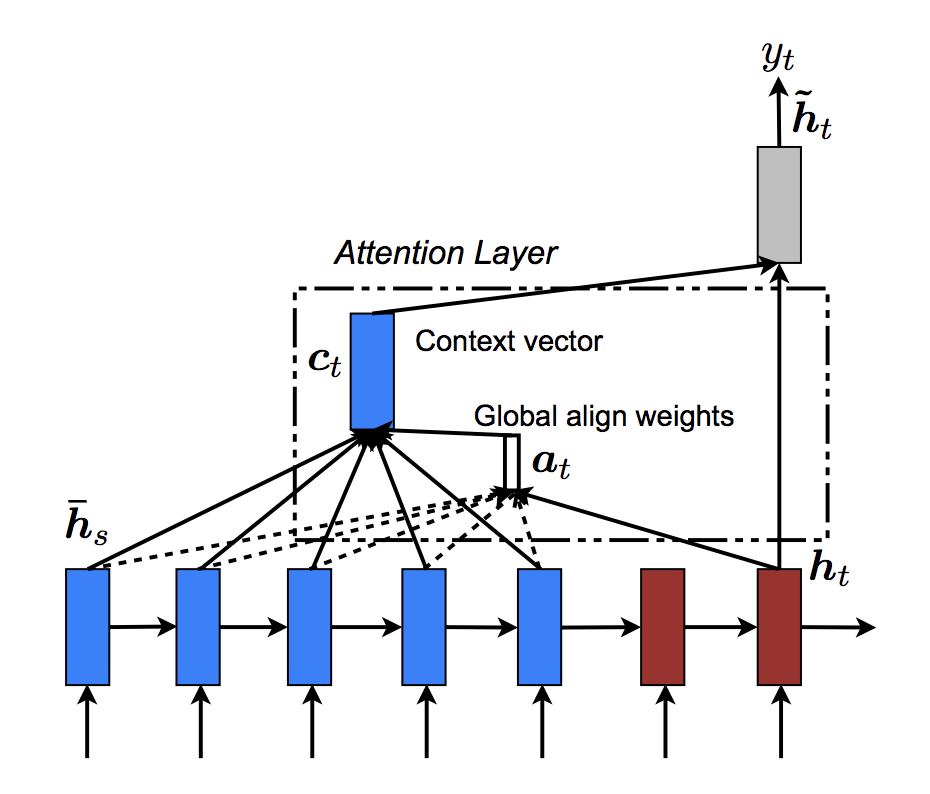
Overall, the Global attention mechanism can be summarized by the following figure. Note that we will implement the “Attention Layer” as a separate nn.Module called Attn. The output of this module is a softmax normalized weights tensor of shape (batch_size, 1, max_length).

# Luong attention layer
class Attn(nn.Module):
    def __init__(self, method, hidden_size):
        super(Attn, self).__init__()
        self.method = method
        if self.method not in ['dot', 'general', 'concat']:
            raise ValueError(self.method, "is not an appropriate attention method.")
        self.hidden_size = hidden_size
        if self.method == 'general':
            self.attn = nn.Linear(self.hidden_size, hidden_size)
        elif self.method == 'concat':
            self.attn = nn.Linear(self.hidden_size * 2, hidden_size)
            self.v = nn.Parameter(torch.FloatTensor(hidden_size))

    def dot_score(self, hidden, encoder_output):
        return torch.sum(hidden * encoder_output, dim=2)

    def general_score(self, hidden, encoder_output):
        energy = self.attn(encoder_output)
        return torch.sum(hidden * energy, dim=2)

    def concat_score(self, hidden, encoder_output):
        energy = self.attn(torch.cat((hidden.expand(encoder_output.size(0), -1, -1), encoder_output), 2)).tanh()
        return torch.sum(self.v * energy, dim=2)

    def forward(self, hidden, encoder_outputs):
        # Calculate the attention weights (energies) based on the given method
        if self.method == 'general':
            attn_energies = self.general_score(hidden, encoder_outputs)
        elif self.method == 'concat':
            attn_energies = self.concat_score(hidden, encoder_outputs)
        elif self.method == 'dot':
            attn_energies = self.dot_score(hidden, encoder_outputs)

        # Transpose max_length and batch_size dimensions
        attn_energies = attn_energies.t()

        # Return the softmax normalized probability scores (with added dimension)
        return F.softmax(attn_energies, dim=1).unsqueeze(1)

Now that we have defined our attention submodule, we can implement the actual decoder model. For the decoder, we will manually feed our batch one time step at a time. This means that our embedded word tensor and GRU output will both have shape (1, batch_size, hidden_size).

Computation Graph:

1. Get embedding of current input word.

2. Forward through unidirectional GRU.

3. Calculate attention weights from the current GRU output from (2).

4. Multiply attention weights to encoder outputs to get new “weighted sum” context vector.

5. Concatenate weighted context vector and GRU output using Luong eq. 5.

6. Predict next word using Luong eq. 6 (without softmax).

7. Return output and final hidden state.

Inputs:

• input_step: one time step (one word) of input sequence batch; shape=(1, batch_size)

• last_hidden: final hidden layer of GRU; shape=(n_layers x num_directions, batch_size, hidden_size)

• encoder_outputs: encoder model’s output; shape=(max_length, batch_size, hidden_size)

Outputs:

• output: softmax normalized tensor giving probabilities of each word being the correct next word in the decoded sequence; shape=(batch_size, voc.num_words)

• hidden: final hidden state of GRU; shape=(n_layers x num_directions, batch_size, hidden_size)

class LuongAttnDecoderRNN(nn.Module):
    def __init__(self, attn_model, embedding, hidden_size, output_size, n_layers=1, dropout=0.1):
        super(LuongAttnDecoderRNN, self).__init__()

        # Keep for reference
        self.attn_model = attn_model
        self.hidden_size = hidden_size
        self.output_size = output_size
        self.n_layers = n_layers
        self.dropout = dropout

        # Define layers
        self.embedding = embedding
        self.embedding_dropout = nn.Dropout(dropout)
        self.gru = nn.GRU(hidden_size, hidden_size, n_layers, dropout=(0 if n_layers == 1 else dropout))
        self.concat = nn.Linear(hidden_size * 2, hidden_size)
        self.out = nn.Linear(hidden_size, output_size)

        self.attn = Attn(attn_model, hidden_size)

    def forward(self, input_step, last_hidden, encoder_outputs):
        # Note: we run this one step (word) at a time
        # Get embedding of current input word
        embedded = self.embedding(input_step)
        embedded = self.embedding_dropout(embedded)
        # Forward through unidirectional GRU
        rnn_output, hidden = self.gru(embedded, last_hidden)
        # Calculate attention weights from the current GRU output
        attn_weights = self.attn(rnn_output, encoder_outputs)
        # Multiply attention weights to encoder outputs to get new "weighted sum" context vector
        context = attn_weights.bmm(encoder_outputs.transpose(0, 1))
        # Concatenate weighted context vector and GRU output using Luong eq. 5
        rnn_output = rnn_output.squeeze(0)
        context = context.squeeze(1)
        concat_input = torch.cat((rnn_output, context), 1)
        concat_output = torch.tanh(self.concat(concat_input))
        # Predict next word using Luong eq. 6
        output = self.out(concat_output)
        output = F.softmax(output, dim=1)
        # Return output and final hidden state
        return output, hidden

Define Training Procedure

Masked loss

Since we are dealing with batches of padded sequences, we cannot simply consider all elements of the tensor when calculating loss. We define maskNLLLoss to calculate our loss based on our decoder’s output tensor, the target tensor, and a binary mask tensor describing the padding of the target tensor. This loss function calculates the average negative log likelihood of the elements that correspond to a 1 in the mask tensor.

def maskNLLLoss(inp, target, mask):
    nTotal = mask.sum()
    crossEntropy = -torch.log(torch.gather(inp, 1, target.view(-1, 1)).squeeze(1))
    loss = crossEntropy.masked_select(mask).mean()
    loss = loss.to(device)
    return loss, nTotal.item()

Single training iteration

The train function contains the algorithm for a single training iteration (a single batch of inputs).

We will use a couple of clever tricks to aid in convergence:

• The first trick is using teacher forcing. This means that at some probability, set by teacher_forcing_ratio, we use the current target word as the decoder’s next input rather than using the decoder’s current guess. This technique acts as training wheels for the decoder, aiding in more efficient training. However, teacher forcing can lead to model instability during inference, as the decoder may not have a sufficient chance to truly craft its own output sequences during training. Thus, we must be mindful of how we are setting the teacher_forcing_ratio, and not be fooled by fast convergence.

• The second trick that we implement is gradient clipping. This is a commonly used technique for countering the “exploding gradient” problem. In essence, by clipping or thresholding gradients to a maximum value, we prevent the gradients from growing exponentially and either overflow (NaN), or overshoot steep cliffs in the cost function.

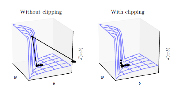
Image source: Goodfellow et al. Deep Learning. 2016. https://www.deeplearningbook.org/

Sequence of Operations:

1. Forward pass entire input batch through encoder.

2. Initialize decoder inputs as SOS_token, and hidden state as the encoder’s final hidden state.

3. Forward input batch sequence through decoder one time step at a time.

4. If teacher forcing: set next decoder input as the current target; else: set next decoder input as current decoder output.

5. Calculate and accumulate loss.

6. Perform backpropagation.

7. Clip gradients.

8. Update encoder and decoder model parameters.

Note

PyTorch’s RNN modules (RNN, LSTM, GRU) can be used like any other non-recurrent layers by simply passing them the entire input sequence (or batch of sequences). We use the GRU layer like this in the encoder. The reality is that under the hood, there is an iterative process looping over each time step calculating hidden states. Alternatively, you ran run these modules one time-step at a time. In this case, we manually loop over the sequences during the training process like we must do for the decoder model. As long as you maintain the correct conceptual model of these modules, implementing sequential models can be very straightforward.

def train(input_variable, lengths, target_variable, mask, max_target_len, encoder, decoder, embedding,
          encoder_optimizer, decoder_optimizer, batch_size, clip, max_length=MAX_LENGTH):

    # Zero gradients
    encoder_optimizer.zero_grad()
    decoder_optimizer.zero_grad()

    # Set device options
    input_variable = input_variable.to(device)
    lengths = lengths.to(device)
    target_variable = target_variable.to(device)
    mask = mask.to(device)

    # Initialize variables
    loss = 0
    print_losses = []
    n_totals = 0

    # Forward pass through encoder
    encoder_outputs, encoder_hidden = encoder(input_variable, lengths)

    # Create initial decoder input (start with SOS tokens for each sentence)
    decoder_input = torch.LongTensor([[SOS_token for _ in range(batch_size)]])
    decoder_input = decoder_input.to(device)

    # Set initial decoder hidden state to the encoder's final hidden state
    decoder_hidden = encoder_hidden[:decoder.n_layers]

    # Determine if we are using teacher forcing this iteration
    use_teacher_forcing = True if random.random() < teacher_forcing_ratio else False

    # Forward batch of sequences through decoder one time step at a time
    if use_teacher_forcing:
        for t in range(max_target_len):
            decoder_output, decoder_hidden = decoder(
                decoder_input, decoder_hidden, encoder_outputs
            )
            # Teacher forcing: next input is current target
            decoder_input = target_variable[t].view(1, -1)
            # Calculate and accumulate loss
            mask_loss, nTotal = maskNLLLoss(decoder_output, target_variable[t], mask[t])
            loss += mask_loss
            print_losses.append(mask_loss.item() * nTotal)
            n_totals += nTotal
    else:
        for t in range(max_target_len):
            decoder_output, decoder_hidden = decoder(
                decoder_input, decoder_hidden, encoder_outputs
            )
            # No teacher forcing: next input is decoder's own current output
            _, topi = decoder_output.topk(1)
            decoder_input = torch.LongTensor([[topi[i][0] for i in range(batch_size)]])
            decoder_input = decoder_input.to(device)
            # Calculate and accumulate loss
            mask_loss, nTotal = maskNLLLoss(decoder_output, target_variable[t], mask[t])
            loss += mask_loss
            print_losses.append(mask_loss.item() * nTotal)
            n_totals += nTotal

    # Perform backpropatation
    loss.backward()

    # Clip gradients: gradients are modified in place
    _ = nn.utils.clip_grad_norm_(encoder.parameters(), clip)
    _ = nn.utils.clip_grad_norm_(decoder.parameters(), clip)

    # Adjust model weights
    encoder_optimizer.step()
    decoder_optimizer.step()

    return sum(print_losses) / n_totals

Training iterations

It is finally time to tie the full training procedure together with the data. The trainIters function is responsible for running n_iterations of training given the passed models, optimizers, data, etc. This function is quite self explanatory, as we have done the heavy lifting with the train function.

One thing to note is that when we save our model, we save a tarball containing the encoder and decoder state_dicts (parameters), the optimizers’ state_dicts, the loss, the iteration, etc. Saving the model in this way will give us the ultimate flexibility with the checkpoint. After loading a checkpoint, we will be able to use the model parameters to run inference, or we can continue training right where we left off.

def trainIters(model_name, voc, pairs, encoder, decoder, encoder_optimizer, decoder_optimizer, embedding, encoder_n_layers, decoder_n_layers, save_dir, n_iteration, batch_size, print_every, save_every, clip, corpus_name, loadFilename):

    # Load batches for each iteration
    training_batches = [batch2TrainData(voc, [random.choice(pairs) for _ in range(batch_size)])
                      for _ in range(n_iteration)]

    # Initializations
    print('Initializing ...')
    start_iteration = 1
    print_loss = 0
    if loadFilename:
        start_iteration = checkpoint['iteration'] + 1

    # Training loop
    print("Training...")
    for iteration in range(start_iteration, n_iteration + 1):
        training_batch = training_batches[iteration - 1]
        # Extract fields from batch
        input_variable, lengths, target_variable, mask, max_target_len = training_batch

        # Run a training iteration with batch
        loss = train(input_variable, lengths, target_variable, mask, max_target_len, encoder,
                     decoder, embedding, encoder_optimizer, decoder_optimizer, batch_size, clip)
        print_loss += loss

        # Print progress
        if iteration % print_every == 0:
            print_loss_avg = print_loss / print_every
            print("Iteration: {}; Percent complete: {:.1f}%; Average loss: {:.4f}".format(iteration, iteration / n_iteration * 100, print_loss_avg))
            print_loss = 0

        # Save checkpoint
        if (iteration % save_every == 0):
            directory = os.path.join(save_dir, model_name, corpus_name, '{}-{}_{}'.format(encoder_n_layers, decoder_n_layers, hidden_size))
            if not os.path.exists(directory):
                os.makedirs(directory)
            torch.save({
                'iteration': iteration,
                'en': encoder.state_dict(),
                'de': decoder.state_dict(),
                'en_opt': encoder_optimizer.state_dict(),
                'de_opt': decoder_optimizer.state_dict(),
                'loss': loss,
                'voc_dict': voc.__dict__,
                'embedding': embedding.state_dict()
            }, os.path.join(directory, '{}_{}.tar'.format(iteration, 'checkpoint')))

Define Evaluation

After training a model, we want to be able to talk to the bot ourselves. First, we must define how we want the model to decode the encoded input.

Greedy decoding

Greedy decoding is the decoding method that we use during training when we are NOT using teacher forcing. In other words, for each time step, we simply choose the word from decoder_output with the highest softmax value. This decoding method is optimal on a single time-step level.

To facilite the greedy decoding operation, we define a GreedySearchDecoder class. When run, an object of this class takes an input sequence (input_seq) of shape (input_seq length, 1), a scalar input length (input_length) tensor, and a max_length to bound the response sentence length. The input sentence is evaluated using the following computational graph:

Computation Graph:

1. Forward input through encoder model.

2. Prepare encoder’s final hidden layer to be first hidden input to the decoder.

3. Initialize decoder’s first input as SOS_token.

4. Initialize tensors to append decoded words to.

5. Iteratively decode one word token at a time:

   1. Forward pass through decoder.

   2. Obtain most likely word token and its softmax score.

   3. Record token and score.

   4. Prepare current token to be next decoder input.

6. Return collections of word tokens and scores.

class GreedySearchDecoder(nn.Module):
    def __init__(self, encoder, decoder):
        super(GreedySearchDecoder, self).__init__()
        self.encoder = encoder
        self.decoder = decoder

    def forward(self, input_seq, input_length, max_length):
        # Forward input through encoder model
        encoder_outputs, encoder_hidden = self.encoder(input_seq, input_length)
        # Prepare encoder's final hidden layer to be first hidden input to the decoder
        decoder_hidden = encoder_hidden[:decoder.n_layers]
        # Initialize decoder input with SOS_token
        decoder_input = torch.ones(1, 1, device=device, dtype=torch.long) * SOS_token
        # Initialize tensors to append decoded words to
        all_tokens = torch.zeros([0], device=device, dtype=torch.long)
        all_scores = torch.zeros([0], device=device)
        # Iteratively decode one word token at a time
        for _ in range(max_length):
            # Forward pass through decoder
            decoder_output, decoder_hidden = self.decoder(decoder_input, decoder_hidden, encoder_outputs)
            # Obtain most likely word token and its softmax score
            decoder_scores, decoder_input = torch.max(decoder_output, dim=1)
            # Record token and score
            all_tokens = torch.cat((all_tokens, decoder_input), dim=0)
            all_scores = torch.cat((all_scores, decoder_scores), dim=0)
            # Prepare current token to be next decoder input (add a dimension)
            decoder_input = torch.unsqueeze(decoder_input, 0)
        # Return collections of word tokens and scores
        return all_tokens, all_scores

Evaluate my text

Now that we have our decoding method defined, we can write functions for evaluating a string input sentence. The evaluate function manages the low-level process of handling the input sentence. We first format the sentence as an input batch of word indexes with batch_size==1. We do this by converting the words of the sentence to their corresponding indexes, and transposing the dimensions to prepare the tensor for our models. We also create a lengths tensor which contains the length of our input sentence. In this case, lengths is scalar because we are only evaluating one sentence at a time (batch_size==1). Next, we obtain the decoded response sentence tensor using our GreedySearchDecoder object (searcher). Finally, we convert the response’s indexes to words and return the list of decoded words.

evaluateInput acts as the user interface for our chatbot. When called, an input text field will spawn in which we can enter our query sentence. After typing our input sentence and pressing Enter, our text is normalized in the same way as our training data, and is ultimately fed to the evaluate function to obtain a decoded output sentence. We loop this process, so we can keep chatting with our bot until we enter either “q” or “quit”.

Finally, if a sentence is entered that contains a word that is not in the vocabulary, we handle this gracefully by printing an error message and prompting the user to enter another sentence.

def evaluate(encoder, decoder, searcher, voc, sentence, max_length=MAX_LENGTH):
    ### Format input sentence as a batch
    # words -> indexes
    indexes_batch = [indexesFromSentence(voc, sentence)]
    # Create lengths tensor
    lengths = torch.tensor([len(indexes) for indexes in indexes_batch])
    # Transpose dimensions of batch to match models' expectations
    input_batch = torch.LongTensor(indexes_batch).transpose(0, 1)
    # Use appropriate device
    input_batch = input_batch.to(device)
    lengths = lengths.to(device)
    # Decode sentence with searcher
    tokens, scores = searcher(input_batch, lengths, max_length)
    # indexes -> words
    decoded_words = [voc.index2word[token.item()] for token in tokens]
    return decoded_words


def evaluateInput(encoder, decoder, searcher, voc):
    input_sentence = ''
    while(1):
        try:
            # Get input sentence
            input_sentence = input('> ')
            # Check if it is quit case
            if input_sentence == 'q' or input_sentence == 'quit': break
            # Normalize sentence
            input_sentence = normalizeString(input_sentence)
            # Evaluate sentence
            output_words = evaluate(encoder, decoder, searcher, voc, input_sentence)
            # Format and print response sentence
            output_words[:] = [x for x in output_words if not (x == 'EOS' or x == 'PAD')]
            print('Bot:', ' '.join(output_words))

        except KeyError:
            print("Error: Encountered unknown word.")

Run Model

Finally, it is time to run our model!

Regardless of whether we want to train or test the chatbot model, we must initialize the individual encoder and decoder models. In the following block, we set our desired configurations, choose to start from scratch or set a checkpoint to load from, and build and initialize the models. Feel free to play with different model configurations to optimize performance.

# Configure models
model_name = 'cb_model'
attn_model = 'dot'
#attn_model = 'general'
#attn_model = 'concat'
hidden_size = 500
encoder_n_layers = 2
decoder_n_layers = 2
dropout = 0.1
batch_size = 64

# Set checkpoint to load from; set to None if starting from scratch
loadFilename = None
checkpoint_iter = 4000
#loadFilename = os.path.join(save_dir, model_name, corpus_name,
#                            '{}-{}_{}'.format(encoder_n_layers, decoder_n_layers, hidden_size),
#                            '{}_checkpoint.tar'.format(checkpoint_iter))


# Load model if a loadFilename is provided
if loadFilename:
    # If loading on same machine the model was trained on
    checkpoint = torch.load(loadFilename)
    # If loading a model trained on GPU to CPU
    #checkpoint = torch.load(loadFilename, map_location=torch.device('cpu'))
    encoder_sd = checkpoint['en']
    decoder_sd = checkpoint['de']
    encoder_optimizer_sd = checkpoint['en_opt']
    decoder_optimizer_sd = checkpoint['de_opt']
    embedding_sd = checkpoint['embedding']
    voc.__dict__ = checkpoint['voc_dict']


print('Building encoder and decoder ...')
# Initialize word embeddings
embedding = nn.Embedding(voc.num_words, hidden_size)
if loadFilename:
    embedding.load_state_dict(embedding_sd)
# Initialize encoder & decoder models
encoder = EncoderRNN(hidden_size, embedding, encoder_n_layers, dropout)
decoder = LuongAttnDecoderRNN(attn_model, embedding, hidden_size, voc.num_words, decoder_n_layers, dropout)
if loadFilename:
    encoder.load_state_dict(encoder_sd)
    decoder.load_state_dict(decoder_sd)
# Use appropriate device
encoder = encoder.to(device)
decoder = decoder.to(device)
print('Models built and ready to go!')

Run Training

Run the following block if you want to train the model.

First we set training parameters, then we initialize our optimizers, and finally we call the trainIters function to run our training iterations.

# Configure training/optimization
clip = 50.0
teacher_forcing_ratio = 1.0
learning_rate = 0.0001
decoder_learning_ratio = 5.0
n_iteration = 4000
print_every = 1
save_every = 500

# Ensure dropout layers are in train mode
encoder.train()
decoder.train()

# Initialize optimizers
print('Building optimizers ...')
encoder_optimizer = optim.Adam(encoder.parameters(), lr=learning_rate)
decoder_optimizer = optim.Adam(decoder.parameters(), lr=learning_rate * decoder_learning_ratio)
if loadFilename:
    encoder_optimizer.load_state_dict(encoder_optimizer_sd)
    decoder_optimizer.load_state_dict(decoder_optimizer_sd)

# If you have cuda, configure cuda to call
for state in encoder_optimizer.state.values():
    for k, v in state.items():
        if isinstance(v, torch.Tensor):
            state[k] = v.cuda()

for state in decoder_optimizer.state.values():
    for k, v in state.items():
        if isinstance(v, torch.Tensor):
            state[k] = v.cuda()

# Run training iterations
print("Starting Training!")
trainIters(model_name, voc, pairs, encoder, decoder, encoder_optimizer, decoder_optimizer,
           embedding, encoder_n_layers, decoder_n_layers, save_dir, n_iteration, batch_size,
           print_every, save_every, clip, corpus_name, loadFilename)

Run Evaluation

To chat with your model, run the following block.

# Set dropout layers to eval mode
encoder.eval()
decoder.eval()

# Initialize search module
searcher = GreedySearchDecoder(encoder, decoder)

# Begin chatting (uncomment and run the following line to begin)
# evaluateInput(encoder, decoder, searcher, voc)

Conclusion

That’s all for this one, folks. Congratulations, you now know the fundamentals to building a generative chatbot model! If you’re interested, you can try tailoring the chatbot’s behavior by tweaking the model and training parameters and customizing the data that you train the model on.

Check out the other tutorials for more cool deep learning applications in PyTorch!